Problems tagged with "SVMs"

Let \(X = \{\nvec{x}{i}, y_i\}\) be a data set of \(n\) points where each \(\nvec{x}{i}\in\mathbb R^d\).

Let \(Z = \{\nvec{z}{i}, y_i\}\) be the data set obtained from the original by standardizing each feature. That is, if a matrix were created with the \(i\)th row being \(\nvec{z}{i}\), then the mean of each column would be zero, and the variance would be one.

Suppose that \(X\) and \(Z\) are both linearly-separable. Suppose Hard-SVMs \(H_1\) and \(H_2\) are trained on \(X\) and \(Z\), respectively.

True or False: \(H_1(\nvec{x}{i}) = H_2(\nvec{z}{i})\) for each \(i = 1, \ldots, n\).

The image below shows a linear prediction function \(H\) along with a data set; the ``\(\times\)'' points have label +1 while the ``\(\circ\)'' points have label -1. Also shown are the places where the output of \(H\) is 0, 1, and -1.

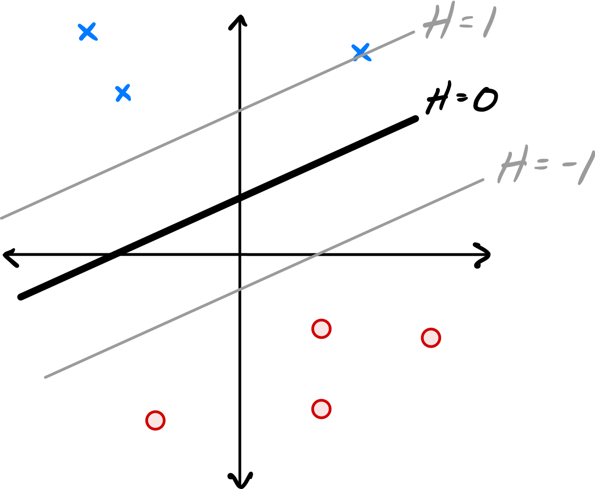
True or False: \(H\) could have been learned by training a Hard-SVM on this data set.

Suppose a data set \(\mathcal D\) is linearly separable. True or False: a Hard-SVM trained of \(\mathcal D\) is guaranteed to achieve 100\% training accuracy.

The image below shows a linear prediction function \(H\) along with a data set; the ``\(\times\)'' points have label +1 while the ``\(\circ\)'' points have label -1. Also shown are the places where the output of \(H\) is 0, 1, and -1.

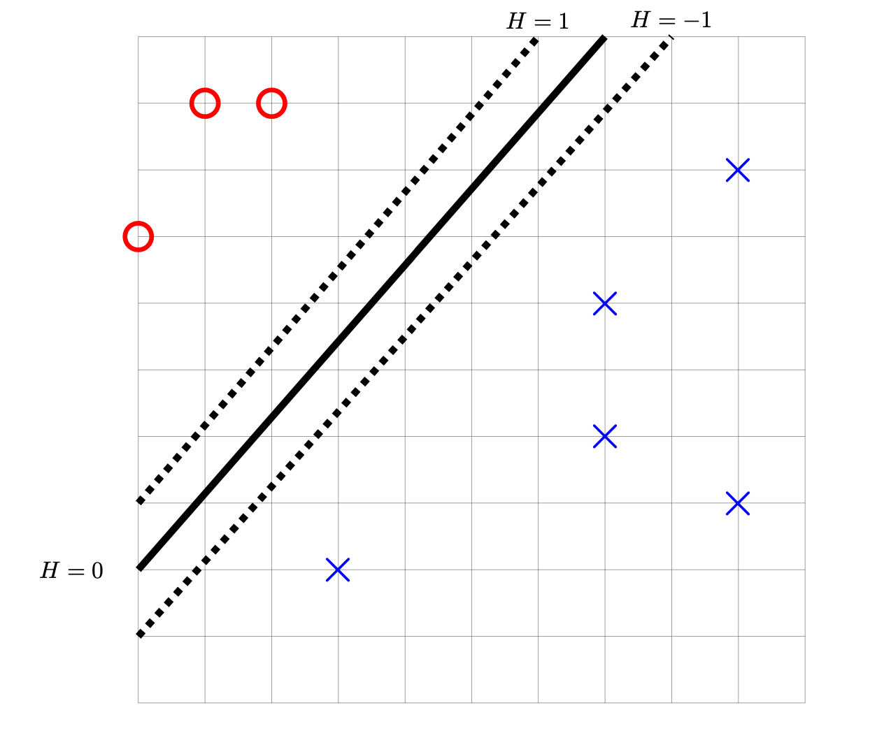
True or False: \(H\) could have been learned by training a Hard-SVM on this data set.

In lecture, we saw that SVMs minimize the (regularized) risk with respect to the hinge loss. Now recall, the 0-1 loss, which was defined in lecture as:

Consider the data set shown below. The points marked with ``+'' have label +1, while the ``\(\circ\)'' points have label -1. Shown are the places where a linear prediction function \(H\) is equal to zero (the thick solid line), 1, and -1 (the dotted lines). Each cell of the grid is 1 unit by 1 unit. The origin is not specified (it is not necssary to know the absolute coordinates of any points for this problem).

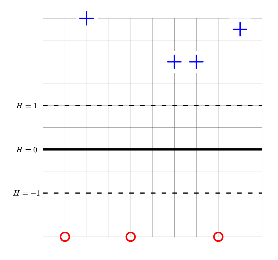
Suppose that the weight vector \(\vec w\) of the linear prediction function \(w_0 + w_1 x_1 + w_2 x_2\) shown above is \((6, 0, \frac{1}{2})^T\). This weight vector is not the solution to the Hard SVM problem.

What weight vector is the solution of the Hard SVM problem for this data set?

\((3, 0, \frac{1}{4})^T\) Show Answer

Let \(\mathcal X\) be a binary classification data set \((\nvec{x}{1}, y_1), \ldots, (\nvec{x}{n}, y_n)\), where each \(\nvec{x}{i}\in\mathbb R^d\) and each \(y_i \in\{-1, 1\}\). Suppose that the data in \(\mathcal X\) is linearly separable.

Let \(\vec w_{\text{svm}}\) be the weight vector of the hard-margin support vector machine (SVM) trained on \(\mathcal X\). Let \(\vec w_{\text{lsq}}\) be the weight vector of the least squares classifier trained on \(\mathcal X\).

True or False: it must be the case that \(\vec w_{\text{svm}} = \vec w_{\text{lsq}}\).

Recall that the Soft-SVM optimization problem is given by

where \(\vec w\) is the weight vector, \(\vec\xi\) is a vector of slack variables, and \(C\) is a regularization parameter.

The two pictures below show as dashed lines the decision boundaries that result from training a Soft-SVM on the same data set using two different regularization parameters: \(C_1\) and \(C_2\).

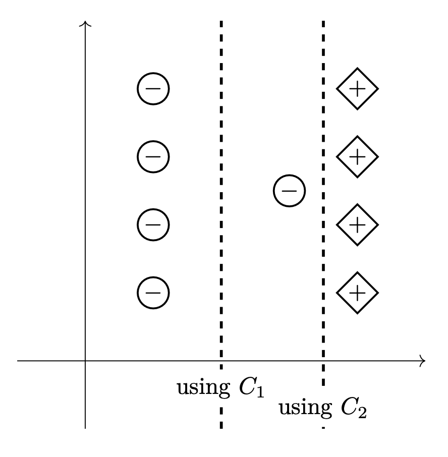
True or False: \(C_1 < C_2\).

Consider the data set shown below. The points marked with ``+'' have label +1, while the ``\(\circ\)'' points have label -1. Shown are the places where a linear prediction function \(H\) is equal to zero (the thick solid line), 1, and -1 (the dotted lines). Each cell of the grid is 1 unit by 1 unit. The origin is not specified (it is not necssary to know the absolute coordinates of any points for this problem).

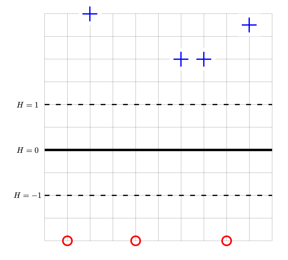
Let \(\vec w'\) be the parameter vector corresponding to prediction function \(H\) shown above. Let \(R(\vec w)\) be the risk with respect to the hinge loss on this data. True or False: the gradient of \(R\) evaluated at \(\vec w'\) is \(\vec 0\).